11. Two Meanings of Probability

11.1. Overview

This lecture illustrates two distinct interpretations of a probability distribution

• A frequentist interpretation as relative frequencies anticipated to occur in a large IID. sample

• A Bayesian interpretation as a personal opinion (about a parameter or list of parameters) after seeing a collection of observations

We recommend watching this video about hypothesis testing within the frequentist approach

After you watch that video, please watch the following video on the Bayesian approach to constructing coverage intervals

After you are familiar with the material in these videos, this lecture uses the Socratic method to help consolidate your understanding of the different questions that are answered by

• a frequentist confidence interval

• a Bayesian coverage interval

We do this by inviting you to write some Python code.

It would be especially useful if you tried doing this after each question that we pose for you, before proceeding to read the rest of the lecture.

We provide our own answers as the lecture unfolds, but you’ll learn more if you try writing your own code before reading and running ours.

Code for answering questions:

To answer our coding questions, we’ll start with some imports

import numpy as np
import pandas as pd
import matplotlib.pyplot as plt
from scipy.stats import binom
import scipy.stats as st

Matplotlib is building the font cache; this may take a moment.

Empowered with these Python tools, we’ll now explore the two meanings described above.

11.2. Frequentist Interpretation

Consider the following classic example.

The random variable \(X \) takes on possible values \(k = 0, 1, 2, \ldots, n\) with probabilities

\[ \mathbb{P}\{X = k \mid \theta\} = \left(\frac{n!}{k! (n-k)!} \right) \theta^k (1-\theta)^{n-k} \]

where the fixed parameter \(\theta \in (0,1)\).

This is called the binomial distribution.

Here

• \(\theta\) is the probability that one toss of a coin will be a head, an outcome that we encode as \(Y = 1\).

• \(1 -\theta\) is the probability that one toss of the coin will be a tail, an outcome that we denote \(Y = 0\).

• \(X\) is the total number of heads that came up after flipping the coin \(n\) times.

Consider the following experiment:

Take \(I\) independent sequences of \(n\) independent flips of the coin

Notice the repeated use of the adjective independent:

• we use it once to describe that we are drawing \(n\) independent times from a Bernoulli distribution with parameter \(\theta\) to arrive at one draw from a Binomial distribution with parameters \(\theta,n\).

• we use it again to describe that we are then drawing \(I\) sequences of \(n\) coin draws.

Let \(y_h^i \in \{0, 1\}\) be the realized value of \(Y\) on the \(h\)th flip during the \(i\)th sequence of flips.

Let \(\sum_{h=1}^n y_h^i\) denote the total number of times heads come up during the \(i\)th sequence of \(n\) independent coin flips.

Let \(f_k\) record the fraction of samples of length \(n\) for which \(\sum_{h=1}^n y_h^i = k\):

\[ f_k^I = \frac{\textrm{number of samples of length n for which } \sum_{h=1}^n y_h^i = k}{ I} \]

The probability \(\mathbb{P}\{X = k \mid \theta\}\) answers the following question:

• As \(I\) becomes large, in what fraction of \(I\) independent draws of \(n\) coin flips should we anticipate \(k\) heads to occur?

As usual, a law of large numbers justifies this answer.

Exercise 11.1

1. Please write a Python class to compute \(f_k^I\)

2. Please use your code to compute \(f_k^I, k = 0, \ldots , n\) and compare them to \(\mathbb{P}\{X = k \mid \theta\}\) for various values of \(\theta, n\) and \(I\)

3. With the Law of Large Numbers in mind, use your code to describe the relationship between \(f_k^I\) and \(\mathbb{P}\{X = k \mid \theta\}\) as \(I\) grows

Solution

Here is one solution:

class Frequentist:

    def __init__(self, θ, n, I, rng=None):
        self.θ, self.n, self.I = θ, n, I
        self.rng = rng or np.random.default_rng()

    def binomial(self, k):
        '''Compute the theoretical probability.'''
        self.P = binom.pmf(k, self.n, self.θ)

    def draw(self):
        '''Draw n independent flips for I sequences.'''
        θ, n, I = self.θ, self.n, self.I
        sample = self.rng.random((I, n))
        self.Y = (sample <= θ).astype(int)

    def compute_fk(self, k):
        '''Compute f_k^I for a given k.'''
        head_counts = np.sum(self.Y, axis=1)
        self.f_kI = np.sum(head_counts == k) / self.I

    def compare(self):
        '''Compute and print the comparison.'''
        self.draw()
        rows = []
        for k in range(self.n + 1):
            self.binomial(k)
            self.compute_fk(k)
            rows.append([k, self.P, self.f_kI])
        return pd.DataFrame(
            rows, columns=['k', 'Theoretical', 'Frequentist']
        ).set_index('k')

rng = np.random.default_rng(123)
θ, n, k, I = 0.7, 20, 10, 1_000_000

freq = Frequentist(θ, n, I, rng=rng)

freq.compare()

	Theoretical	Frequentist
k
0	3.486784e-11	0.000000
1	1.627166e-09	0.000000
2	3.606885e-08	0.000000
3	5.049639e-07	0.000000
4	5.007558e-06	0.000006
5	3.738977e-05	0.000041
6	2.181070e-04	0.000203
7	1.017833e-03	0.001020
8	3.859282e-03	0.003833
9	1.200665e-02	0.012198
10	3.081708e-02	0.030651
11	6.536957e-02	0.065378
12	1.143967e-01	0.114649
13	1.642620e-01	0.164867
14	1.916390e-01	0.191439
15	1.788631e-01	0.178644
16	1.304210e-01	0.130448
17	7.160367e-02	0.071426
18	2.784587e-02	0.027683
19	6.839337e-03	0.006680
20	7.979227e-04	0.000834

From the table above, can you see the law of large numbers at work?

Let’s do some more calculations.

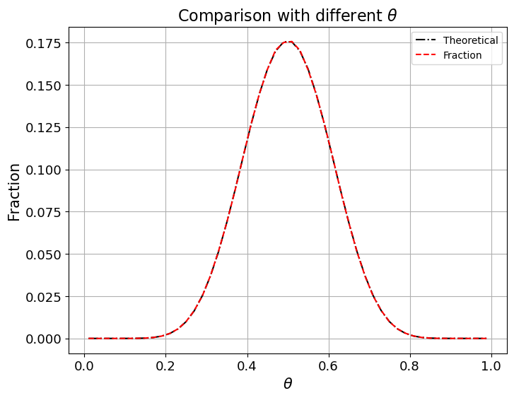
Comparison with different \(\theta\)

Now we fix

\[ n=20, k=10, I=1,000,000 \]

We’ll vary \(\theta\) from \(0.01\) to \(0.99\) and plot outcomes against \(\theta\).

rng = np.random.default_rng(234)
θ_low, θ_high, n_thetas = 0.01, 0.99, 50
thetas = np.linspace(θ_low, θ_high, n_thetas)
P = []
f_kI = []
for i in range(n_thetas):
    freq = Frequentist(thetas[i], n, I, rng=rng)
    freq.binomial(k)
    freq.draw()
    freq.compute_fk(k)
    P.append(freq.P)
    f_kI.append(freq.f_kI)

fig, ax = plt.subplots(figsize=(8, 6))
ax.grid()
ax.plot(thetas, P, 'k-.', label='Theoretical')
ax.plot(thetas, f_kI, 'r--', label='Fraction')
ax.set_title(r'Comparison with different $\theta$',
             fontsize=16)
ax.set_xlabel(r'$\theta$', fontsize=15)
ax.set_ylabel('Fraction', fontsize=15)
ax.tick_params(labelsize=13)
ax.legend()
plt.show()

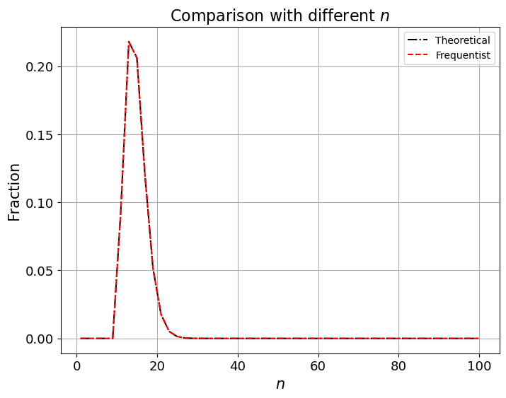
Comparison with different \(n\)

Now we fix \(\theta=0.7, k=10, I=1,000,000\) and vary \(n\) from \(1\) to \(100\).

Then we’ll plot outcomes.

rng = np.random.default_rng(345)
n_low, n_high, n_ns = 1, 100, 50
ns = np.linspace(n_low, n_high, n_ns, dtype='int')
P = []
f_kI = []
for i in range(n_ns):
    freq = Frequentist(θ, ns[i], I, rng=rng)
    freq.binomial(k)
    freq.draw()
    freq.compute_fk(k)
    P.append(freq.P)
    f_kI.append(freq.f_kI)

fig, ax = plt.subplots(figsize=(8, 6))
ax.grid()
ax.plot(ns, P, 'k-.', label='Theoretical')
ax.plot(ns, f_kI, 'r--', label='Frequentist')
ax.set_title(r'Comparison with different $n$',
             fontsize=16)
ax.set_xlabel(r'$n$', fontsize=15)
ax.set_ylabel('Fraction', fontsize=15)
ax.tick_params(labelsize=13)
ax.legend()
plt.show()

Comparison with different \(I\)

Now we fix \(\theta=0.7, n=20, k=10\) and vary \(\log(I)\) from \(2\) to \(6\).

rng = np.random.default_rng(456)
I_log_low, I_log_high, n_Is = 2, 6, 200
log_Is = np.linspace(I_log_low, I_log_high, n_Is)
Is = np.power(10, log_Is).astype(int)
P = []
f_kI = []
for i in range(n_Is):
    freq = Frequentist(θ, n, Is[i], rng=rng)
    freq.binomial(k)
    freq.draw()
    freq.compute_fk(k)
    P.append(freq.P)
    f_kI.append(freq.f_kI)

fig, ax = plt.subplots(figsize=(8, 6))
ax.grid()
ax.plot(Is, P, 'k-.', label='Theoretical')
ax.plot(Is, f_kI, 'r--', label='Fraction')
ax.set_title(r'Comparison with different $I$',
             fontsize=16)
ax.set_xlabel(r'$I$', fontsize=15)
ax.set_ylabel('Fraction', fontsize=15)
ax.tick_params(labelsize=13)
ax.legend()
plt.show()

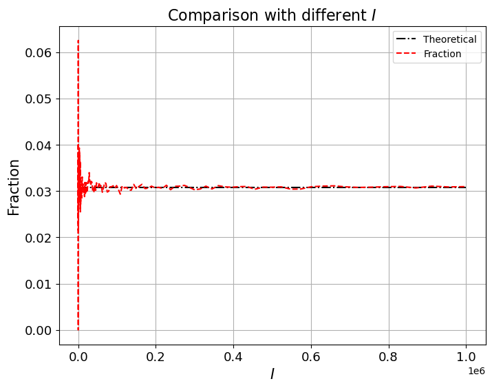
From the above graphs, we can see that \(I\), the number of independent sequences, plays an important role.

When \(I\) becomes larger, the difference between theoretical probability and frequentist estimate becomes smaller.

Also, as long as \(I\) is large enough, changing \(\theta\) or \(n\) does not substantially change the accuracy of the observed fraction as an approximation of \(\mathbb{P}\{X = k \mid \theta\}\).

The Law of Large Numbers is at work here.

For each draw of an independent sequence, \(\mathbb{P}\{X_i = k \mid \theta\}\) is the same, so aggregating all draws forms an IID sequence of a binary random variable \(\rho_{k,i},i=1,2,...I\), with a mean of \(\mathbb{P}\{X = k \mid \theta\}\) and a variance of

\[ \mathbb{P}\{X = k \mid \theta\} \cdot (1-\mathbb{P}\{X = k \mid \theta\}). \]

So, by the LLN, the average of \(\rho_{k,i}\) converges to:

\[ \mathbb{E}[\rho_{k,i}] = \mathbb{P}\{X = k \mid \theta\} = \left(\frac{n!}{k! (n-k)!} \right) \theta^k (1-\theta)^{n-k} \]

as \(I\) goes to infinity.

11.3. Bayesian Interpretation

We again use a binomial distribution.

But now we don’t regard \(\theta\) as being a fixed number.

Instead, we think of it as a random variable.

\(\theta\) is described by a probability distribution.

But now this probability distribution means something different than a relative frequency that we can anticipate to occur in a large IID. sample.

Instead, the probability distribution of \(\theta\) is now a summary of our views about likely values of \(\theta\) either

• before we have seen any data at all, or

• before we have seen more data, after we have seen some data

Thus, suppose that, before seeing any data, you have a personal prior probability distribution with density

\[ p(\theta) = \frac{\theta^{\alpha-1}(1-\theta)^{\beta -1}}{B(\alpha, \beta)} \]

where \(B(\alpha, \beta)\) is a beta function , so that \(p(\theta)\) is the density of a beta distribution with parameters \(\alpha, \beta\).

We can update this prior after observing data using Bayes’ Law (see Probability with Matrices for an introduction).

For a sample of \(n\) coin flips that yields \(k\) heads, the likelihood function is the binomial probability

\[ L(k \mid \theta) = {n \choose k} \theta^k (1-\theta)^{n-k} \]

Applying Bayes’ Law with our beta prior, the posterior density is

\[ p(\theta \mid k) = \frac{L(k \mid \theta) \cdot p(\theta)}{\int_0^1 L(k \mid \theta) \cdot p(\theta) \, d\theta} = \textrm{Beta}(\alpha + k, \, \beta + n - k) \]

So the posterior is also a beta distribution — a consequence of the beta prior being conjugate to the binomial likelihood.

Exercise 11.2

a) Please write down the likelihood function for a single coin flip with outcome \(Y \in \{0, 1\}\).

b) Please write down the posterior distribution for \(\theta\) after observing that single flip.

c) Now pretend that the true value of \(\theta = .4\) and that someone who doesn’t know this has a beta prior distribution with parameters \(\beta = \alpha = .5\). Please write a Python class to simulate this person’s personal posterior distribution for \(\theta\) for a single sequence of \(n\) draws.

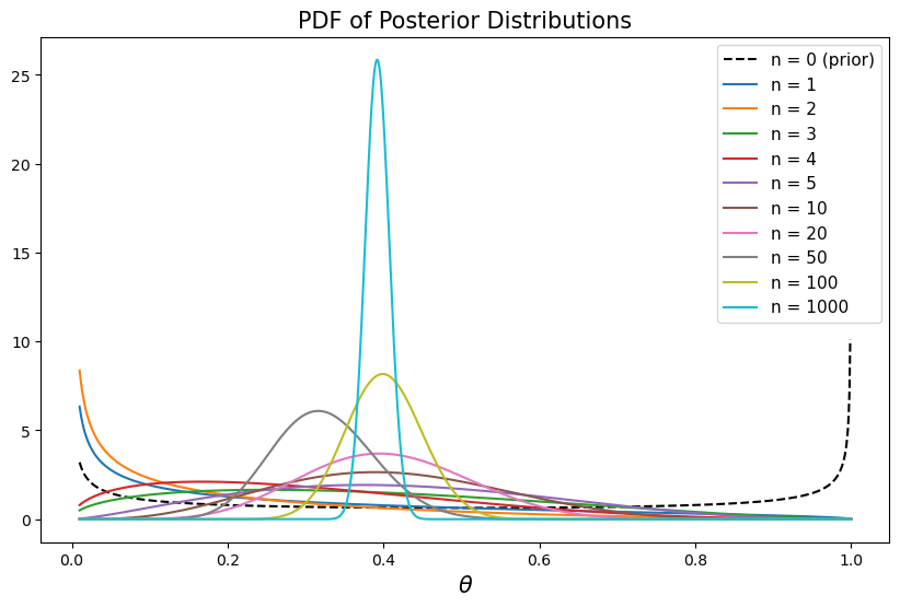
d) Please plot the posterior distribution for \(\theta\) as a function of \(\theta\) as \(n\) grows as \(1, 2, \ldots\).

e) For various \(n\)’s, please describe and compute a Bayesian coverage interval for the interval \([.45, .55]\).

f) Please tell what question a Bayesian coverage interval answers.

g) Please compute the Posterior probability that \(\theta \in [.45, .55]\) for various values of sample size \(n\).

h) Please use your Python class to study what happens to the posterior distribution as \(n \rightarrow + \infty\), again assuming that the true value of \(\theta = .4\), though it is unknown to the person doing the updating via Bayes’ Law.

Solution

a) The likelihood function for a single coin flip with outcome \(Y \in \{0, 1\}\) is

\[ L(Y|\theta) = \theta^Y (1-\theta)^{1-Y} \]

b) By Bayes’ Law, the posterior density for \(\theta\) after observing a single flip \(Y\) is

\[ p(\theta \mid Y) = \frac{L(Y \mid \theta) \cdot p(\theta)}{\int_{0}^{1} L(Y \mid \theta) \cdot p(\theta) \, d\theta} \]

Substituting the likelihood from (a) and the beta prior density, this becomes

\[ p(\theta \mid Y) = \frac{\theta^Y (1-\theta)^{1-Y} \cdot \theta^{\alpha - 1} (1 - \theta)^{\beta - 1} / B(\alpha, \beta)}{\int_{0}^{1} \theta^Y (1-\theta)^{1-Y} \cdot \theta^{\alpha - 1} (1 - \theta)^{\beta - 1} / B(\alpha, \beta) \, d\theta} \]

Collecting powers of \(\theta\) and \((1-\theta)\), we recognize the kernel of a beta density:

\[ p(\theta \mid Y) = \frac{\theta^{Y+\alpha - 1} (1 - \theta)^{1-Y+\beta - 1}}{\int_{0}^{1} \theta^{Y+\alpha - 1} (1 - \theta)^{1-Y+\beta - 1} \, d\theta} \]

which means that

\[ \theta \mid Y \sim \textrm{Beta}(\alpha + Y, \, \beta + (1-Y)) \]

c)

class Bayesian:

    def __init__(self, θ=0.4, n=1_000_000, α=0.5, β=0.5,
                 rng=None):
        '''
        Parameters
        ----------
        θ : Probability of heads on each flip.
        n : Number of flips in the sequence.
        α, β : Parameters of the beta prior on θ.
        rng : NumPy random generator.
        '''
        self.θ, self.n, self.α, self.β = θ, n, α, β
        self.rng = rng or np.random.default_rng()
        self.prior = st.beta(α, β)

    def draw(self):
        '''Simulate a sequence of n coin flips.'''
        array = self.rng.random(self.n)
        self.draws = (array < self.θ).astype(int)

    def form_single_posterior(self, n_obs):
        '''Return the posterior after the first n_obs flips.'''
        heads = self.draws[:n_obs].sum()
        tails = n_obs - heads
        return st.beta(self.α + heads, self.β + tails)

    def form_posterior_series(self, n_obs_list):
        '''Form posteriors for each sample size in n_obs_list.'''
        self.posterior_list = []
        for n_obs in n_obs_list:
            self.posterior_list.append(
                self.form_single_posterior(n_obs)
            )

d)

rng = np.random.default_rng(567)
bayes = Bayesian(rng=rng)
bayes.draw()

n_obs_list = [1, 2, 3, 4, 5, 10, 20, 50,
              100, 1000,
              5000, 10_000, 50_000, 100_000,
              200_000, 300_000]

bayes.form_posterior_series(n_obs_list)

θ_values = np.linspace(0.01, 1, 1000)

fig, ax = plt.subplots(figsize=(10, 6))

ax.plot(θ_values, bayes.prior.pdf(θ_values),
        label='n = 0 (prior)', color='k',
        linestyle='--')

for i, n_obs in enumerate(n_obs_list[:10]):
    posterior = bayes.posterior_list[i]
    ax.plot(θ_values, posterior.pdf(θ_values),
            label=f'n = {n_obs}')

ax.set_title('PDF of Posterior Distributions',
             fontsize=15)
ax.set_xlabel(r"$\theta$", fontsize=15)

ax.legend(fontsize=11)
plt.show()

e)

lower_bound = [post.ppf(0.05) for post in bayes.posterior_list[:10]]
upper_bound = [post.ppf(0.95) for post in bayes.posterior_list[:10]]

interval_df = pd.DataFrame()
interval_df['upper'] = upper_bound
interval_df['lower'] = lower_bound
interval_df.index = n_obs_list[:10]
interval_df = interval_df.T
interval_df

	1	2	3	4	5	10	20	50	100	1000
upper	0.771480	0.569259	0.764466	0.650707	0.739366	0.652678	0.582446	0.434206	0.481969	0.417601
lower	0.001543	0.000868	0.062413	0.046007	0.127776	0.185116	0.237639	0.220799	0.322252	0.366860

As \(n\) increases, we can see that Bayesian coverage intervals narrow and move toward \(0.4\).

f) The Bayesian coverage interval tells the range of \(\theta\) that corresponds to the [\(q_1\), \(q_2\)] quantiles of the cumulative distribution function (CDF) of the posterior distribution.

To construct the coverage interval we first compute a posterior distribution of the unknown parameter \(\theta\).

If the CDF is \(F(\theta)\), then the Bayesian coverage interval \([a,b]\) for the interval \([q_1,q_2]\) is described by

\[ F(a)=q_1,F(b)=q_2 \]

g)

left_value, right_value = 0.45, 0.55

posterior_prob_list = [
    post.cdf(right_value) - post.cdf(left_value)
    for post in bayes.posterior_list
]

fig, ax = plt.subplots(figsize=(8, 5))
ax.plot(posterior_prob_list)
ax.set_title(
    r'Posterior Probability that $\theta$'
    f' Ranges from {left_value:.2f}'
    f' to {right_value:.2f}',
    fontsize=13)
ax.set_xticks(np.arange(0, len(posterior_prob_list), 3))
ax.set_xticklabels(n_obs_list[::3])
ax.set_xlabel('Number of Observations', fontsize=11)

plt.show()

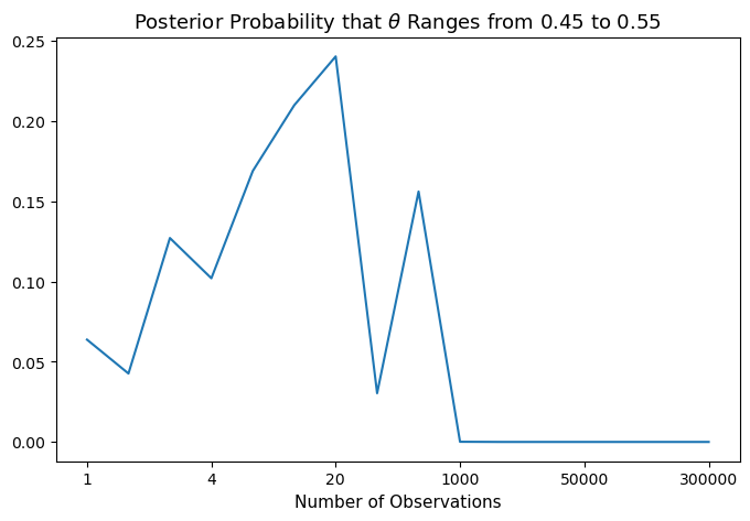
Notice that in the graph above the posterior probability that \(\theta \in [.45, .55]\) exhibits a hump shape as \(n\) increases.

Two opposing forces are at work.

The first force is that the individual adjusts his belief as he observes new outcomes, so his posterior probability distribution becomes more and more realistic, which explains the rise of the posterior probability.

However, \([.45, .55]\) actually excludes the true \(\theta =.4 \) that generates the data.

As a result, the posterior probability drops as larger and larger samples refine his posterior probability distribution of \(\theta\).

The descent seems precipitous only because of the scale of the graph that has the number of observations increasing disproportionately.

When the number of observations becomes large enough, our Bayesian becomes so confident about \(\theta\) that he considers \(\theta \in [.45, .55]\) very unlikely.

That is why we see a nearly horizontal line when the number of observations exceeds 1000.

h) Using the Python class we made above, we can see the evolution of posterior distributions as \(n\) approaches infinity.

fig, ax = plt.subplots(figsize=(10, 6))

for i, n_obs in enumerate(n_obs_list[10:]):
    posterior = bayes.posterior_list[i + 10]
    ax.plot(θ_values, posterior.pdf(θ_values),
            label=f'n = {n_obs:,}')

ax.set_title('PDF of Posterior Distributions', fontsize=15)
ax.set_xlabel(r"$\theta$", fontsize=15)
ax.set_xlim(0.3, 0.5)

ax.legend(fontsize=11)
plt.show()

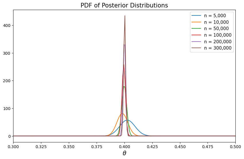
As \(n\) increases, we can see that the probability density functions concentrate on \(0.4\), the true value of \(\theta\).

Here the posterior mean converges to \(0.4\) while the posterior standard deviation converges to \(0\) from above.

To show this, we compute the mean and standard deviation of the posterior distributions.

mean_list = [post.mean() for post in bayes.posterior_list]
std_list = [post.std() for post in bayes.posterior_list]

fig, ax = plt.subplots(1, 2, figsize=(14, 5))

ax[0].plot(mean_list)
ax[0].set_title('Mean of Posterior Distribution',
                fontsize=13)
ax[0].set_xticks(np.arange(0, len(mean_list), 3))
ax[0].set_xticklabels(n_obs_list[::3])
ax[0].set_xlabel('Number of Observations', fontsize=11)

ax[1].plot(std_list)
ax[1].set_title('Std Dev of Posterior Distribution',
                fontsize=13)
ax[1].set_xticks(np.arange(0, len(std_list), 3))
ax[1].set_xticklabels(n_obs_list[::3])
ax[1].set_xlabel('Number of Observations', fontsize=11)

plt.show()

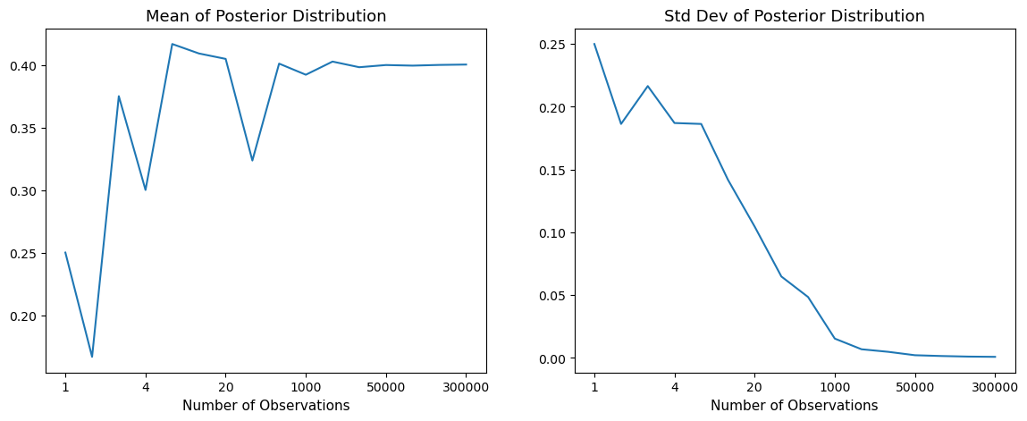
How shall we interpret the patterns above?

The answer is encoded in the Bayesian updating formula derived above.

Recall that after observing \(k\) heads in \(n\) flips, the posterior is \(\textrm{Beta}(\alpha + k, \, \beta + n - k)\).

A beta distribution with parameters \(\alpha\) and \(\beta\) has

• mean \(\frac{\alpha}{\alpha + \beta}\)

• variance \(\frac{\alpha \beta}{(\alpha + \beta)^2 (\alpha + \beta + 1)}\)

Here \(\alpha + k\) can be viewed as the number of successes (prior pseudo-count plus observed heads) and \(\beta + n - k\) as the number of failures.

Since the data are generated with \(\theta = 0.4\), the Law of Large Numbers tells us that, as \(n\) grows, \(k/n \to 0.4\) (see Exercise 11.1).

Consequently, the posterior mean converges to \(0.4\) and the posterior variance shrinks to zero.

upper_bound = [post.ppf(0.95) for post in bayes.posterior_list]
lower_bound = [post.ppf(0.05) for post in bayes.posterior_list]

fig, ax = plt.subplots(figsize=(10, 6))
ax.scatter(np.arange(len(upper_bound)),
           upper_bound, label='95th Quantile')
ax.scatter(np.arange(len(lower_bound)),
           lower_bound, label='5th Quantile')

ax.set_xticks(np.arange(0, len(upper_bound), 2))
ax.set_xticklabels(n_obs_list[::2])
ax.set_xlabel('Number of Observations', fontsize=12)
ax.set_title('Bayesian Coverage Intervals of '
             'Posterior Distributions', fontsize=15)

ax.legend(fontsize=11)
plt.show()

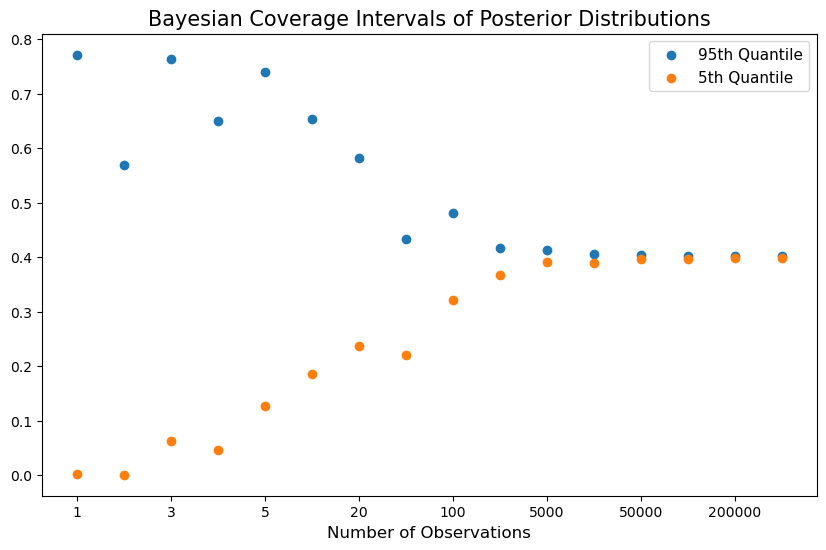
After observing a large number of outcomes, the posterior distribution collapses around \(0.4\).

Thus, the Bayesian statistician comes to believe that \(\theta\) is near \(.4\).

As shown in the figure above, as the number of observations grows, the Bayesian coverage intervals (BCIs) become narrower and narrower around \(0.4\).

However, if you take a closer look, you will find that the centers of the BCIs are not exactly \(0.4\), due to the persistent influence of the prior distribution and the randomness of the simulation path.

11.4. Role of a Conjugate Prior

We have made assumptions that link functional forms of our likelihood function and our prior in a way that has eased our calculations considerably.

In particular, our assumptions that the likelihood function is binomial and that the prior distribution is a beta distribution have the consequence that the posterior distribution implied by Bayes’ Law is also a beta distribution.

So posterior and prior are both beta distributions, albeit ones with different parameters.

When a likelihood function and prior fit together like hand and glove in this way, we can say that the prior and posterior are conjugate distributions.

In this situation, we also sometimes say that we have conjugate prior for the likelihood function \(\mathbb{P}\{X \mid \theta\}\).

Typically, the functional form of the likelihood function determines the functional form of a conjugate prior.

A natural question to ask is why should a person’s personal prior about a parameter \(\theta\) be restricted to be described by a conjugate prior?

Why not some other functional form that more sincerely describes the person’s beliefs?

To be argumentative, one could ask, why should the form of the likelihood function have anything to say about my personal beliefs about \(\theta\)?

A dignified response to that question is, well, it shouldn’t, but if you want to compute a posterior easily you’ll just be happier if your prior is conjugate to your likelihood.

Otherwise, your posterior won’t have a convenient analytical form and you’ll be in the situation of wanting to apply the Markov chain Monte Carlo techniques deployed in Non-Conjugate Priors.

We also apply these powerful methods to approximating Bayesian posteriors for non-conjugate priors in Posterior Distributions for AR(1) Parameters and Forecasting an AR(1) Process.